Nonnegative Autoencoders
My intuition would say that a part-based decomposition should arise naturally within an autoencoder. To encorporate the next image in an image recognition task, it must be more beneficial to have gradient descent being able to navigate towards the optimal set of neural network weights for that image. If not, for each image gradient descent is all the time navigating some kind of common denominator, none of the images are actually properly represented. For each new image that is getting better classified, the other images are classified worse. With a proper decomposition learning the next representation will not interfere with previous representations. Grossberg calls this in Adaptive Resonance Theory (ART) catastrophic forgetting.
Maybe if we train a network long enough this will be the emerging decomposition strategy indeed. However, this is not what is normally found. The different representations get coupled and there is not a decomposition that allows the network to explore different feature dimensions independently.
One of the means to obtain a part-based representation is to force positive or zero weights in a network. In the literature nonnegative matrix factorization can be found. Due to the nonnegativity constraint the features are additive. This leads to a (sparse) basis where through summation “parts” are added up to a “whole” object. For example, faces are built up out of features like eyes, nostrils, mouth, ears, eyebrows, etc.
Sparse Autoencoder with Nonnegativity Constraint
At Louisville university Ehsan Hosseini-Asl (github), Jacek Zurada (who is running for 2019 IEEE president), and Olfa Nasraoui (twitter) studied how nonnegative constraints can be added to an autoencoder in Deep Learning of Part-based Representation of Data Using Sparse Autoencoders with Nonnegativity Constraints (2016).
An autoencoder which has a latent layer that contains a part-based representation, only has a few of the nodes active at a particular input. In other words, such a representation is sparse.
One of the ways a sparse representation can be enforced is to limit the activation of a hidden unit over all data items \(r\). The average activation of a unit is:
\[\hat{p}_j = \frac{1}{m} \sum_{r=1}^m h_j(x^{(r)})\]To make sure that the activation is limited, we can bound \(\hat{p}_j < p\) with \(p\) a small value close to zero.
The usual cost function is just the reconstruction error \(J_E\). Here, we include the activation limitation by adding an additional term:
\[J_{KL}(p || \hat{p}) = \sum_{j=1}^n p \log \frac{p}{\hat{p}_j} + (1-p) \log \frac{1-p}{1-\hat{p}_j}\]We can prevent overfitting by regularization. This can be done by adding noise to the input, dropout, or by penalizing large weights. The latter corresponds to yet another term:
\[J_{O}(W,b) = \frac{1}{2} \sum_{l=1}^2 \sum_{i=1}^{s_l} \sum_{j=1}^{s_{l+1}} \left( w_{ij}^l \right)^2\]The sizes of adjacent layers are indicated by \(s_l\) and \(s_{l+1}\) (and we are limited to \(l\) layers).
The total cost function used by the authors for the sparse autoencoder contains all the above cost functions, each weighted, one by parameter \(\beta\), the other by \(\lambda\).
\[J_{SAE}(W,b) = J_E(W,b) + \beta J_{KL}(p||\hat{p}) + \lambda J_O(W,b)\]To enforce nonnegativity we can introduce a different regularization term:
\[J_{O}(W,b) = \frac{1}{2} \sum_{l=1}^2 \sum_{i=1}^{s_l} \sum_{j=1}^{s_{l+1}} f \left( w_{ij}^l \right)\]For the nonnegative constrained autoencoder the authors suggest:
\[f(w_{ij}) = \begin{cases} w_{ij}^2 & w_{ij} < 0 \\ 0 & \text{otherwise} \end{cases}\]This term penalizes all negative values. All positive values do not contribute to the cost function.
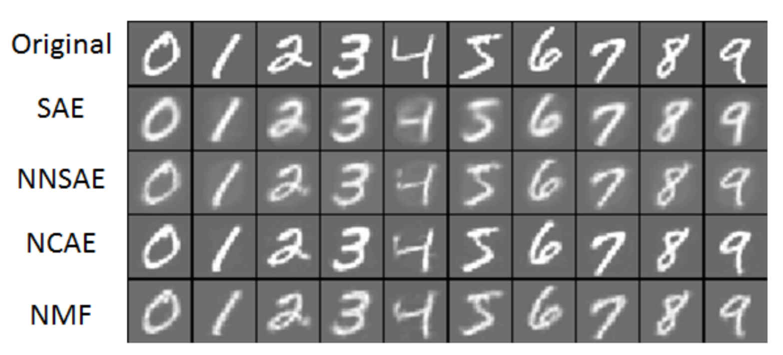
Results
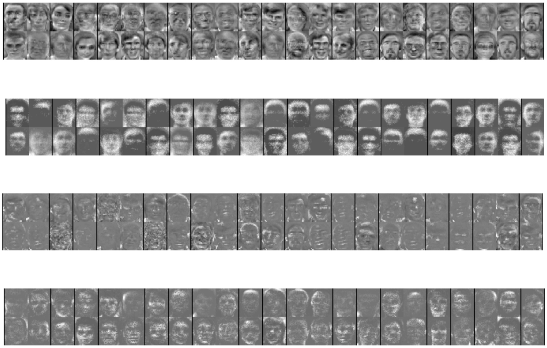
Results are compared between the Sparse Autoencoder (SAE), the Nonnegative Sparse Autoencoder (NNSAE), the Negatively Constrained Autoencoder (NCAE), and Nonnegative Matrix Factorization (NMF).
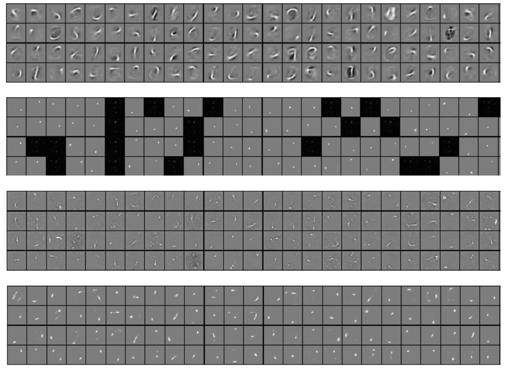
The SAE representation contains negative values (dark pixels). The NNSAE representation has neurons with zero weights (complete black nodes).
The receptive fields learned by NCAE are more sparse than the others. The features from NNSAE and NMF are more local.
Ideas
To really encourage a part-based decomposition it would be best to enforce either very large values or values that are zero. Something like sum over x divided by number of non-zero components with each x nonnegative and maximizing over this.